Exploring a Spatial Wetland Data Resource for the Bow River Basin
Category: Blog
Subject Area: Habitat Monitoring
Published: Jan 27, 2025
Author(s): Guest blogger: Nilo Sinnatamby, Miistakis Institute
Through your 2024 wetland survey responses, we heard about your interest in historical wetland information. This guest blog from the Miistakis Institute introduces the Bow River Region Wetland Datasets and a case study to illustrate their use.
In 2024, the ABMI sent out a survey to learn how wetland practitioners and researchers use existing wetland resources, and what additional resources are needed. Many respondents were interested in historical wetland data but potentially unaware of the wealth of data already available. The Miistakis Institute was invited to provide an overview of the Bow River Regional Wetland Datasets, which include historical wetland data, to demonstrate the datasets' unique features and some suggestions for use through a case study.
What are the Bow River Regional Wetland Datasets?
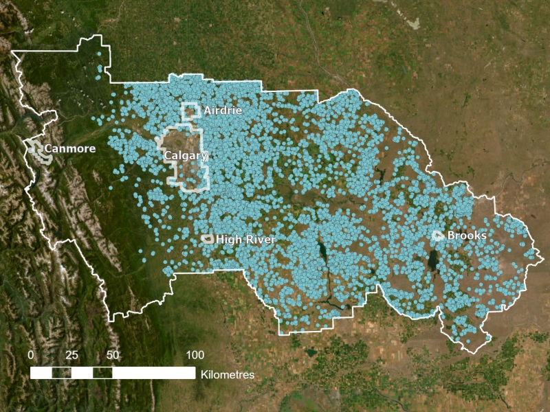
The Bow River Regional Wetland Datasets are wetland-focused spatial resources developed by the Miistakis Institute in partnership with Fiera Biological Consulting and the Bow River Basin Council. The datasets were developed to provide accurate wetland spatial data that is consistent across the Bow Basin–responding to a need expressed by many municipal government participants. To improve utility by municipalities, the spatial extent of the data layers was extended beyond the Bow Basin to match the boundaries of several municipalities.
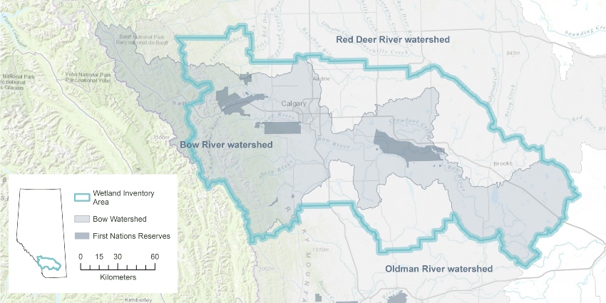
Map showing the extent of the Bow River Regional Wetland Datasets
The datasets include:
 Wetland Inventory:
A spatial representation of wetlands classified according to the Alberta Wetland Classification System and consistent with the Government of Alberta's wetland inventory standards. In this blog post, we refer to this inventory as the 2020 wetland inventory, which reflects the date of most of the imagery used.
Historical Wetland Inventory:
Historical extent of wetlands based on historical air photos from 1949 to 1951.
R estorable Wetland Inventory:
Wetland areas with a high likelihood of human-caused drainage activity that may be eligible for the provincial Wetland Restoration Program.
 Land Cover:
Land classes classified into two hierarchical levels, which integrate the wetland inventory to create a single, seamless product.
How can these datasets help us manage wetlands?
Before we can effectively manage wetlands, we need to know where they are. These four spatial datasets offer unique insights and can be used in a variety of ways to support wetland management. Here are a few examples:
- Using the 2020 wetland inventory, we could ask how many wetlands are located close to roads? Those wetlands tend to have lower water quality and could be prioritized for restoration actions.
- Using the 2020 wetland inventory, we can also quantify how many wetlands are on private vs. public land, which would help us understand the proportion of wetlands that can be accessed more readily for management actions.
- Municipalities, wetland restoration practitioners, and conservation groups could use the potentially restorable wetland inventory to prioritize restoration actions at specific wetlands to maximize the efficient use of restoration dollars. Municipal planners or regional planning bodies could use the land cover dataset for regional land-use planning since it provides a seamless representation of land cover across the region.
For this blog, we took a deeper dive into using the historical and 2020 wetland inventories to look at change in wetland presence over time.
Case Study: How has spatial coverage of wetlands changed over time?
The historical wetland dataset can’t be compared directly to the 2020 wetland dataset. This is especially true at small scales or for individual wetlands. Georectification errors in some of the historical imagery and the less sensitive methods used to capture very small wetlands in historical images contribute to these limitations.
Here’s how we got around these issues:
- Match the spatial footprint: First, we trimmed the 2020 wetland dataset to match the spatial footprint of the historical dataset. Because of poor historical imagery in some areas, the historical dataset does not include the western portion of the study area.
- Exclude very small wetlands: Next, we trimmed wetlands that were smaller than 1000m2—this is about ⅛ of a Canadian football field. This step trimmed 6,822 wetlands from the historical dataset, and 70,833 wetlands from the 2020 wetland dataset.
- Create a grid: To avoid a direct spatial comparison between the datasets at an individual wetland or small scale, we created a hexagonal grid where each cell was 187.2 km2, which is equivalent to two townships. There’s no strict rule for the size of a grid cell or watershed used in this type of assessment—it depends on your specific question and the size of your study area.
Here’s how we compared the grid cells:
- Calculate percentage: We calculated the percentage of each cell that was covered by wetland.
- Standardize: To further reduce potential issues that accompany comparing two differently derived datasets, we standardized the resulting percentages between 0 and 1 for each dataset separately.
- Subtract: We subtracted the standardized historical grid value from the standardized 2020 grid value.
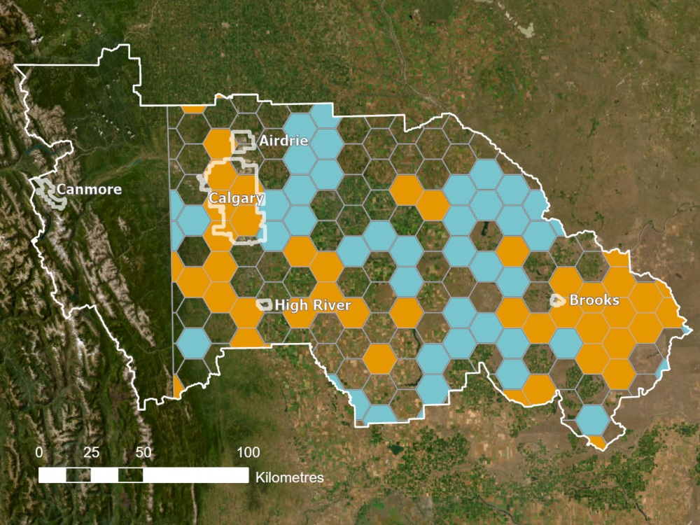
Areas showing the greatest increases in wetland coverage (blue) and greatest decreases in wetland coverage (orange) in the study area. Unshaded areas may have experienced no change in wetland prevalence, or more mild gains or losses. Towns and cities are illustrated to help with orientation.
Here’s how we interpreted the results:
- Separate into quantiles: We divided the resulting values into four quantiles to evaluate the results looking at general patterns.
- Look at areas of most change: We focused on the highest quantile suggesting the most wetland gain (shown in blue) and the lowest quantile suggesting the most wetland loss (shown in orange). This step, and the one prior, were added to ensure we weren't misinterpreting small differences as real changes, since such differences could easily result from comparing datasets derived in different ways.
What we found and potential next steps:
- Both loss and gain: Our comparison suggests that the Bow Basin has likely seen both wetland gains and wetland losses since the mid 1900s. For the purpose of this blog, we stopped our assessment here, however, some next questions could be “what caused those changes?” and “can we use this information to prioritize where wetlands are preserved or restored in the basin to promote ecosystem services and climate resiliency?”.
- A north-south corridor of loss: Our analysis illustrated a north-south corridor near Calgary that has experienced significant wetland loss. This is not surprising since this area has seen the most development and largest population growth within the basin. This information highlights the importance of preserving remaining wetlands or restoring/constructing wetlands within that stretch of the study area.
- Areas of wetland gain: We typically don’t hear many concerns about wetland gain in Alberta, but our findings highlight the importance of considering this type of change as well. Wetland gain could happen as a result of consolidating many small wetlands into one large one, or through irrigation activities. These actions can lead to wetlands transforming from ephemeral to permanent, with changes to hydrological function and implications for the types of species that thrive. This change could also threaten the persistence of naturally saline wetlands that require water flows to be intermittent.
- Remaining uncertainty: Developing and interpreting historical wetland spatial data is a challenge, and probably why these datasets aren’t more common. There is a lot to be gained from this glimpse into our wetland history, but caution should be taken with interpreting this dataset. This resource should be used to help prioritize areas for further investigation, but no actions should be undertaken or conclusions made without ground-truthing.
There's More to Explore!
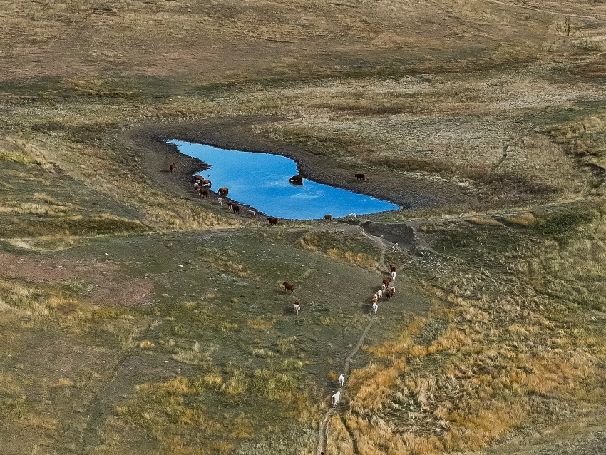
Here’s a peek at the restorable basin layer (left) and photo of one in real life (right). Restorable basins are those identified as having a high likelihood of receiving Wetland Replacement Program funding because they appeared to have been previously, partially or entirely drained.
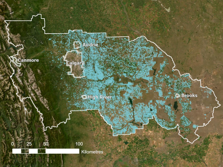
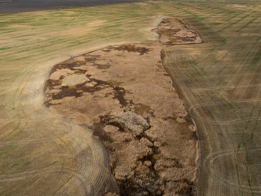
Here’s a peek at disturbed wetlands within the 2020 wetland inventory shown in blue (left). Disturbed wetlands are defined as low-lying depressional areas that are likely wetland basins but have been altered by agricultural activity. The image on the right shows an example of a disturbed wetland.
You can learn more about the datasets, explore a spatial viewer and other resources, and download the datasets here!
Acknowledgements
Miistakis Institute would like to thank The City of Calgary and an anonymous funder, Fiera Biological Consulting, the BRBC, and many other participants who have contributed to the development and refinement of these products.